

Transit planners often ask: how many jobs can someone reach by transit in under an hour? The answer reveals where the network falls short — and where improvements could unlock real access. It’s also a surprisingly hard technical problem, especially when you want to answer it not just from one starting location at one time of day, but across every neighborhood and throughout the day in a city or region.
At Via, we write software that helps transit planners answer these kinds of hard questions. For example, a planner might want to increase frequency on one line, but to stay within budget, may need to reduce it on another. By showing how changes affect access to jobs, schools, healthcare, and other important destinations, planners can make smarter tradeoffs — maximizing impact within their budget.
This post walks through how we rebuilt our transit access feature to scale from a single-point calculation to a full-region system, cutting the runtime from polynomial to constant time in a key step. The approach we landed on also improves how we model the distribution of resources in the real world, making our access analysis more accurate.
The “area-overlap” method.
How would you calculate how many jobs are reachable from a given location at a particular starting time within 60 minutes by transit? In our single-point calculation, we generated an isochrone — a multi-polygon covering all reachable locations within a time limit. To estimate job access in the U.S., we’ll use the Census LEHD, which reports the number of jobs per census block. The “area-overlap” method calculates the number of jobs by intersecting the isochrone with each job polygon, assigning jobs from each job polygon in proportion to the area of that polygon covered by the isochrone.
This works fine for one location. But what if you want to do that for every neighborhood in a city? Our single-point tool couldn’t keep up. Scaling it exposed an unexpected bottleneck.
Let’s walk through these steps in more detail:
Inputs:
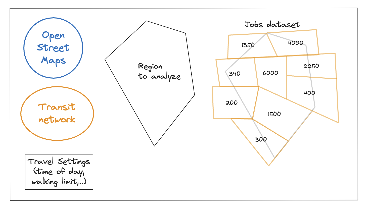
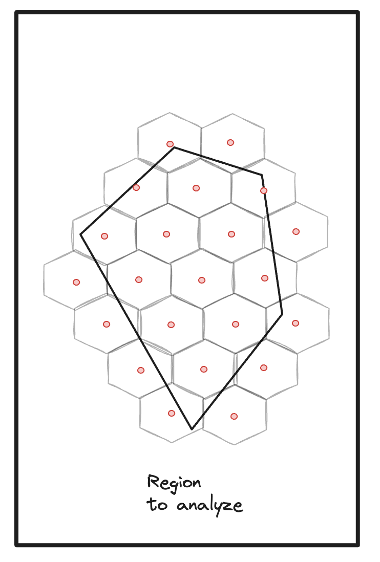
Step 1: Partition region, select centroids as origins.
Step 2: Construct graph.

Step 3: Per origin, we:
Step 3a: Run Dijkstra’s Algorithm from that origin to find all nodes accessible within 60 minutes.

Step 3b: For partially covered street segments (i.e., segments where only one side was reached in the time limit), walk along the segment to find exact stopping point.

Step 3c: Calculate isochrone representing the "area" accessed by generating an alphashape from the accessed points.

Step 3d: determine percent overlap with jobs dataset polygons to calculate jobs accessed.
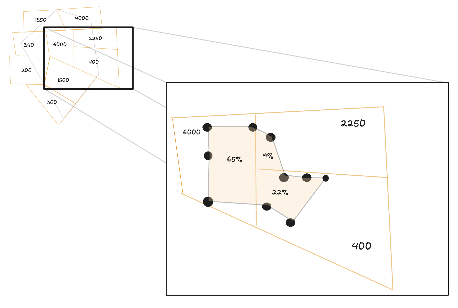
Jobs accessed from this origin = (0.65 * 6000) + (0.09 * 2250) + (0.22 * 400) = 4190
Performance analysis of area-overlap method.
Running the area-overlap method in San Francisco, on a subset of origins (300), it took 4 minutes to calculate accessibility for San Francisco’s Muni service. With that performance, scaling to 30,000 origins like we have in Vancouver would take on the order of 8 hours to calculate. Thus, we wanted to address performance to enable users to iterate more quickly on their transit plans, and to manage infrastructure cost. Measuring the performance in San Francisco gave us clear areas to improve on in future iterations:
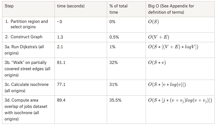
Graph construction and running Dijkstra’s for each origin was quite fast. It turned out that all of the steps after Dijkstra's were where we were spending most of our time: 'walking' to translate from intersections to street edge coverage, computing the isochrone, and the area-overlap calculation for each origin.
Improving performance with the “segment assignment” method.
The key thing to take away from the performance analysis of the area-overlap method is that we’re doing a lot in the loop per origin: specifically, a lot of things related to the jobs polygons and the isochrone. What if we assigned jobs to street segments derived from Open Street Map (OSM) instead?
Intuitively, this is a good idea — things like jobs, grocery stores, libraries, and other desirable destinations are located on streets. For a single access measure, like jobs, we could build a mapping from street segment ID to number of jobs accessible on that street segment. Then, when we want to know the number of jobs accessible from a given origin, if we had the street segment IDs that were accessed, we could look up the number of jobs accessed per street segment and sum them up to get the total. We’ll also consider partial access - that is, if our transit rider can access only 50% of a given street segment, we say they get 50% of the jobs on that street segment.
That mapping from street segment ID to number of jobs accessible on that street segment can be precalculated, since it does not depend on the origin. Once you have the street segment ids, finding the number of jobs accessed just becomes an $$O(1)$$ lookup. In other words, with precomputation, we can take the key step from polynomial time to constant time.
Here’s what the new algorithm looks like in more detail. We start with the same inputs, and steps 1 and 2 (partition region, build graph) are the same. From there, we:
Step 3: Assign jobs to OSM segments.

Step 4: Per origin, we:
Step 4a: Run Dijkstra's from that origin to find all nodes accessible within 60 minutes.

Step 4b: For partially covered street segments (i.e., segments where only one side was reached in the time limit), walk along the segment to find exact stopping point.
Step 4c: Determine percent accessed of each segment.
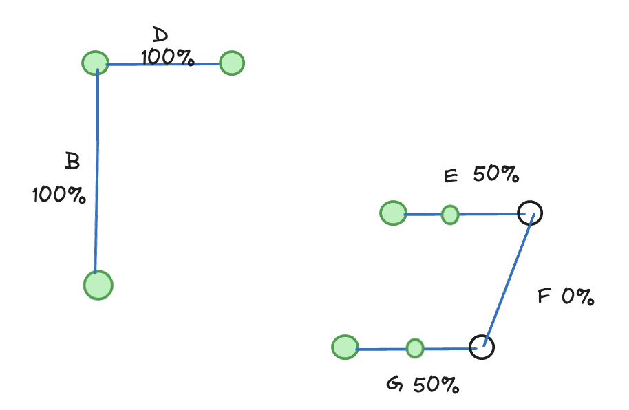
Step 4d: Combine with the jobs per segment.
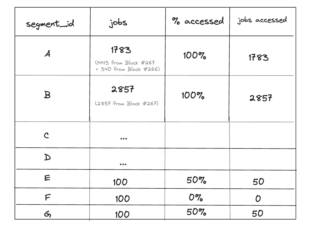
Jobs accessed from this origin = 1783 + 2857 + 50 + 50 = 4740
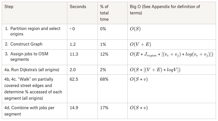
Performance analysis of the segment assignment method.
In the San Francisco test of 300 origins, using the segment assignment method instead of the area overlap method resulted in cutting the runtime by more than half, leaving the “walk on partially covered street segments” step as the most computationally expensive step overall. The cost of the precomputation, while non-trivial, is amortized by running over a large number of origins.
Summary of approaches.
The easiest way to see the performance difference is to notice that the amount of transformation required in the area overlap is higher - for each origin, we need to go from the accessed points, to the isochrone, then do an expensive intersection on each job polygon. In segment assignment, we have a precalculated lookup table of segment ID, and we can get segment IDs accessed per origin just by looking up the segment IDs associated with each accessed point.

The kicker: “segment assignment” is more accurate.
The LEHD and many other job datasets aggregate jobs into polygons. When we use the area overlap method, we’re treating the jobs as evenly distributed across the entire area of the polygon. When the road network is fairly dense, this is a fine assumption, but it breaks down when the street is less dense. The traveler we’re modeling can’t actually walk off the road, which means some of those jobs are distributed to areas inaccessible to them. In truth, it’s more likely that jobs are distributed on the road, because that is how people are able to travel to the job in the first place.
So how do the two approaches actually compare in the real world, and when they differ, what does that mean? In most cases, the two methods produce results within 5% of each other. When there is a meaningful difference, the result from segment assignment aligns better with what we expect from an accessibility analysis. Let’s look at one class of issue to understand this better.
Transit clusters.
A key problem with the area-overlap method is it can overstate access. Fundamentally, the isochrone is translating from points to a multipolygon, resulting in inferring access. The alphashape algorithm effectively shrink-wraps the points to obtain the isochrone, with the parameter (alpha) controlling how tight the shrink-wrap is. As a way of visualizing access, this is a good representation to the extent that access varies smoothly in space. But, the transit network, along with a hard time cutoff of 60 minutes, creates jumps in access - points that are much more accessible than their neighbors.
In this example visualized below, a rider is starting from a point on the transit network outside of Dresden’s city center. The points accessible within 60 minutes are the blue circles, while the red polygon is the isochrone calculated from those points. The blue circles are centered around bus stops - so we have these isolated regions of access. In particular, notice that the region in the bottom of the image (the red area between the bus stops) is not accessible within 60 minutes, though it is within the isochrone. The segment assignment method won't count that red region in the bottom of the image, as it was not accessed, which is more accurate.

Impact.
This work enabled Via to offer the Network Jane feature in Remix to all of our customers, with high performance, reliability, and cost to operate. As a result of using the segment assignment method, we are now able to compute accessibility for 30,000 origins in Vancouver in 2 hours of total compute time. We further improved performance by parallelizing the computation into groups of 500 origins to achieve a balance of benefit from amortization against other factors like peak memory usage. This has many benefits: it enables us to offer this feature at the scale we can with manageable infrastructure costs, and the faster runtime gives transit planners a tight feedback loop, in line with what they expect from the rest of the Remix product experience.
The most meaningful impact is on transit riders - over 300 cities across the world have used this feature as an input into their transit planning processes, enabling them to make more informed decisions about transit access.
Conclusion.
Some of my favorite experiences at Via involve connecting my work to real-world impacts, and continuing to expand my domain knowledge about transit and urban development. The initial insight that assigning jobs to the road network would result in a big performance win was quite a surprise. Finding a performance win that also improved the accuracy of the calculation helped me gain a deeper appreciation of the problem space, and gratitude that I get to work on interesting problems that have a positive impact.
We’re hiring!
Want to work on an engineering team where you can build domain knowledge of transit in close collaboration with transit planners to build solutions that otherwise would not be possible to imagine? Join us!
Appendix (Explanation of Big-O Analysis).
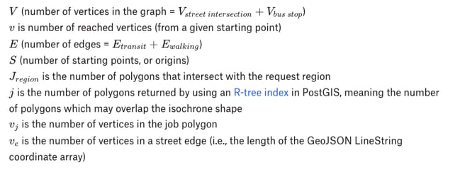
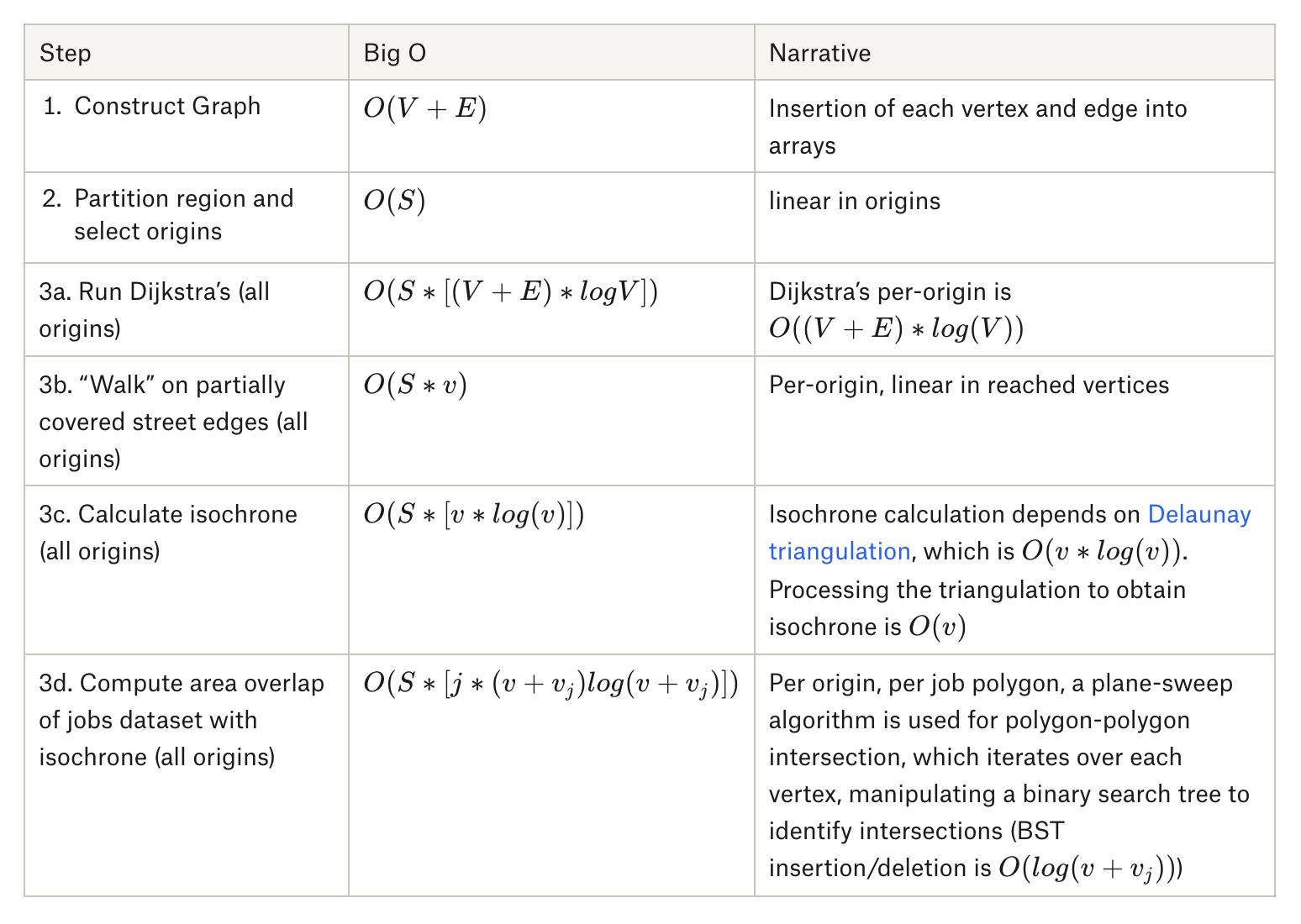
Area Overlap Big-O Analysis explained.
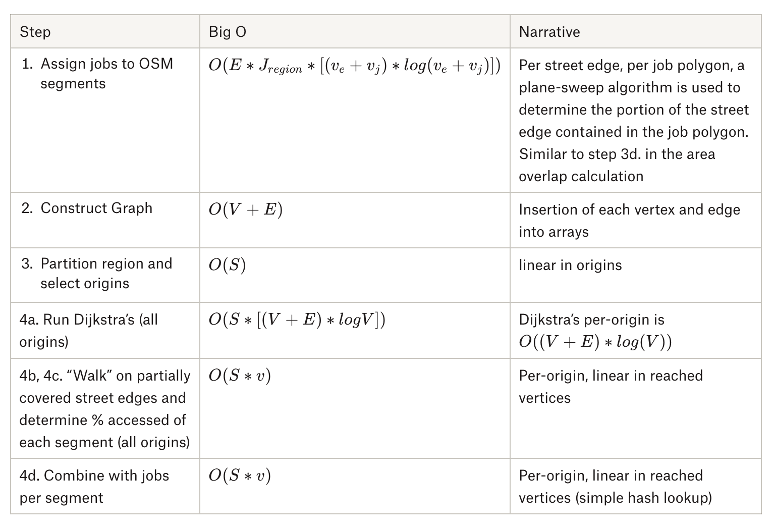
Segment assignment Big-O Analysis explained.


.png?width=71&height=47&name=Sioux%20Falls%20Webinar%20(6).png)